
A Brief Explanation on Adversarial Attack
The core implementation of the neural network is feedforward and backpropagation. Feedforward passes a series of inputs enter the layer, and these inputs are multiplied by the weights. Each value is then added together to get a sum of the weighted input values. It often works with activation functions to scale the classification sensitivity in each neuron.
If you are not familiar with deep learning and neural networks, I highly recommend you to read the previous post: Implementing Neural Networks from Scratch
 Ex10si0n
Backpropagation is for computing the gradients rapidly. In short, what backpropagation does for us is gradient (slope in higher dimensions) calculation. The procedure is straightforward; by adjusting the weights and biases throughout the network, the desired output could be produced from the network. For example, if the output neuron is 0, adjust the weights and biases inside the network to get an output closer to 0. This process is done by minimizing the loss, which needs to be descent by referencing the gradient on the loss function on each parameter (i.e., weights and biases) of every single neuron in the network.
Calculating the gradient in backpropagation could be influenced by each input data X. Usually, the parameters (weights and biases) in the network are adjusted according to the gradient calculated in backpropagation to minimize the loss function. Inversely, the loss is more considerable when the parameters are adjusted to maximize the loss function by going up in the opposite direction.
Adversarial Attacks
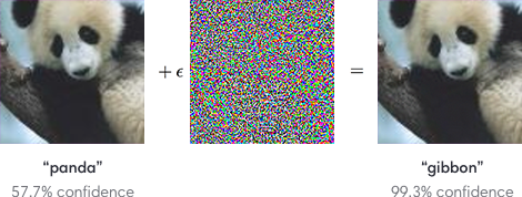
The adversarial vulnerability of deep neural networks has attracted considerable attention in recent years. The adversarial attack is a technique that can deviate the results of Neural Network models to produce wrong predictions—for example, shown in Figure 1, consider that we have a photo of a panda and a CNN model that can accurately categorize a panda image as a label of class “panda”. Adversarial attack techniques (e.g., Fast Gradient Sign Method, 1-pixel attack, and PGD-based attack) can produce a perturbed panda image, called adversarial examples, based on the panda image given and parameters from the CNN classifier. The difference between the adversarial example and the original image from the dataset is hard to observe by human perception. Nevertheless, the CNN classifier wrongly classifies the perturbed image of the panda as other targets, like a gibbon, as a result.
Types of Adversarial Attacks
From the perspective of result achieving, adversarial attacks can be classified into two categories — targeted attacks and untargeted attacks. The targeted attack aims to make the model misclassify a specific class to another given class (target class). On the other hand, the untargeted attack does not have a target class; the goal is simply to make the target model misclassify that specific class.
From the perspective of the right of accessing model parameters, there are white box and black box attacks. A white box attack is one where everything about the deployed model is known, such as inputs, model structure, and specific model internals like weights or coefficient values. In most cases, this means explicitly that the developers have the right to access the internal gradient values of the model. Some researchers also include knowing the entire training data set in white box attacks. Conversely, a black box attack is one where they only know the model inputs and query for output labels or confidence scores.
FGSM Adversarial Attack
One of the most popular methods is the Fast Gradient Sign Method (FGSM) introduced by Ian Goodfellow et al. to create adversarial examples. The paper showed that the FGSM attacks could result in 89.4% misidentification (97.6% confidence) on the original model.
The method of FGSM aims to alternate the input of a deep learning model to a maximum loss using the gradients from backpropagation. Assume that a neural network with intrinsic parameters (weights and biases of each neuron) and the loss function of that neural network is. FGSM algorithm calculates the partial deviation of the loss function to get the direction (sign) to maximum loss increment and add the direction multiplied by the variable (usually a tiny floating number) to each input. Equation 1 describes the mathematical representation of this procedure.
$$x_{adv} = x + \epsilon \times sign(\nabla_xJ(\theta, X, Y))$$
Linear Explanation of Adversarial Examples
Commonly, digital images often use 8 bits per pixel for storing the data, so all information below the atomic size is discarded. Because the precision of the features is limited, the classifier could not give a disparate classification under two input $x$ and $\widetilde{x} = x + \eta$ if every element of the perturbation $\eta$ is smaller than the atomic size. As long as $\max(\eta) < \epsilon$ where $\epsilon$ is small enough to be discarded by the classifier, we expect the classifier to assign the same class to $x$ and $\hat{x}$. Hence the dot product between $w$ and $x$, $\widetilde{x}$
$$w^\top\widetilde{x} = w^\top x+w^\top \eta$$
If $w$ has $n$ dimensions and the average magnitude of an element of the weight vector is $m$, by assigning $\eta = \text{sign}(w)$ where $\text{sign}(x) = +1$ for all $x>0$ and $\text{sign}(x) = -1$ for all $x<0$, then the weighted input $w^\top \widetilde{x}$ will grow by $\epsilon m n$. For high dimensional problems, if we make many infinitesimal changes to the $x$ that adds up to one significant change to the output.
Adversarial Training
Since adversarial examples $\widetilde{x}$ are generated by the input data and the model parameters to make a misclassification to the classifier. However, it is intuitively that if we label the $\widetilde{x}$ to its original class and retrain the model on those examples and their correct labels, this fine-tuning approach by numerous adversarial examples will make the model more robust against adversarial attacks.
In 2019, Tasnim et al. [https://arxiv.org/abs/2105.12106] proposed a data augmentation approach by introducing InvFGSM adversarial learning attack techniques for medical image segmentation, which achieved higher accuracy and robustness
In 2022, Xie et al. [https://arxiv.org/abs/1911.09665] introduced AdvProp (Adversarial Propagation) to improve the recognition accuracy of original data using separate batches for original data and adversarial examples generated by PGD attacks. Their framework achieved 85.2% classification accuracy in ImageNet using adversarial training technique and has a 0.7% growth higher than vanilla training.
According to the literature, adversarial training is a plausible way of enhancing the robustness of a model and a possible way to increase model performance, such as accuracy and AUC, which needs further research and experiments.